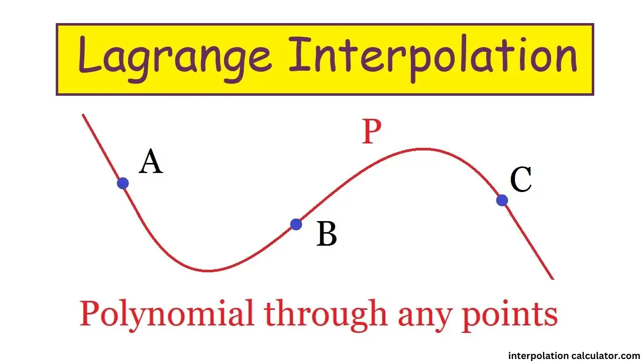
Introduction
What is Lagrange Interpolation:
Lagrange interpolation is a numerical method which is used to approximate a function that passes through a given set of points. The difference is that, unlike linear interpolation, it fits a polynomial of degree n-1, where n is the number of data points. This feature makes it better suited for complex datasets.
How Lagrange Interpolation Works:
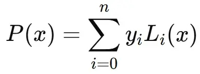
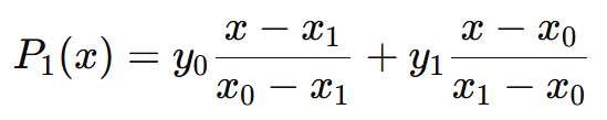
For a given set n data points (x0,y0), (x1, y1),…, (xn,yn), the Lagrange polynomial is given by:
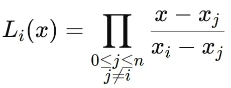
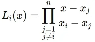
Where Li (x) is the Lagrange basis polynomial, defined as
- Here, P(x) is the interpolated polynomial.
- yi are the known values of the function at xi
- Li (x) is the Lagrange basis polynomial for each data point.
Applications:
Computer Graphics:
It’s used in texture mapping and rendering, which enables smooth transitions.
Data Estimation:
It’s used in datasets where gaps can be filled with great accuracy.
Predictive Modeling:
This interpolation technique is commonly used in weather forecasting and in other fields such as economics to model trends.
Advantages and Limitations:
| Advantages | Limitations |
|---|---|
| Ability to fit a single polynomial to multiple data values. | With a big dataset, the polynomial can become complex leading to oscillations also known as Runge’s phenomenon. |
| It can provide exact results at a given point. | Requires significant computational resources. |
| Accurate for small data. |
Example 1:
The following data points are given, (1,2), (3,6), (4,5). We want to find the polynomial P(x) that passes through these points.
Solution:
The formula is
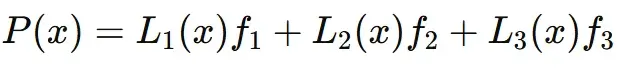
Where Li(x) are the Lagrange basis polynomials and fi are the function values at known points.
Each basis polynomial Li(x) is:
(x1, y1) = (1,2)
(x2, y2) = (3,6)
(x3, y3) = (4,5)
Now, we find each Li(x):
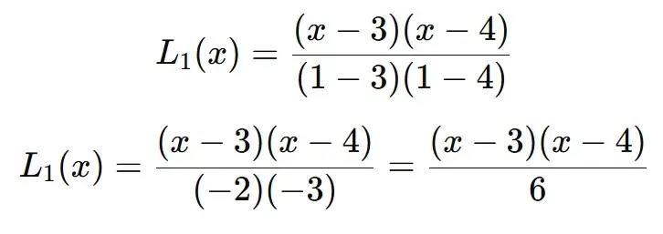
Finding L1(x):
For L1(x), we exclude x1 =1:
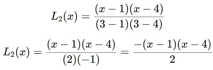
Finding L2(x):
For L2(x), we exclude x2 =3
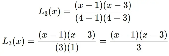
Finding L3(x):
For L3(x), we exclude x3 =4
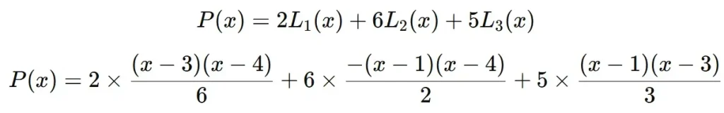
Now we calculate P(x):
To calculate P(x), we multiply each basis polynomial by its corresponding function value and add them.
The formula becomes:
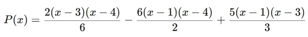
Simplifying:
Simply further to get the final interpolating polynomial.
This is the Lagrange interpolating polynomial passing through the points (1,2), (3,6), (4,5).
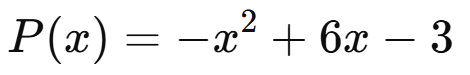
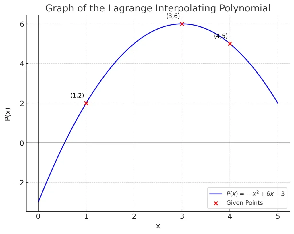
Here you can see the Lagrange interpolating polynomial passing through the points (1,2), (3,6), (4,5).
Lagrange vs Newton Interpolation:
There are some differences between the two interpolation techniques and each has its advantages. You can see the differences in detail in the table below.
| Properties | Lagrange | Newton |
| Method | Uses Lagrange basis polynomials. | Uses divided differences to construct the polynomial. |
| Computational Resources | More resources are needed to compute | Resource friendly. |
| Flexibility | Polynomial must be calculated again when adding new data | It doesn’t need recalculation when adding a new data point. |
| Stability | Susceptible to instability with large datasets. | More stable for large datasets. |
It works well when the dataset is fixed because for each new dataset, recomputing the entire polynomial is required. If the dataset is constantly being updated, then Newton interpolation is more suitable.
Lagrange vs Spline Interpolation:
| Properties | Lagrange | Spline |
| Method | A single polynomial is made from the dataset. | Many low-degree polynomials are made for approximation. |
| Accuracy | High accuracy for small dataset | High accuracy with small and big datasets. |
| Degree of Polynomial | The degree of polynomials increases with more data points. | Can use cubic or quadratic polynomials which keeps from getting overly complicated. |
| Stability | Oscillations may occur between points for large datasets. | The smooth curve is generated for large datasets. |
Against Spline interpolation, Lagrange is only comparable when the dataset is small, for large datasets, Spline interpolation is better suited as it does not suffer from excessive oscillations as Lagrange does.
Lagrange vs Linear Interpolation:
| Properties | Lagrange | Linear |
| Method | Uses a single polynomial to connect the data points. | Connected the two nearest data points with a straight line. |
| Accuracy | More accurate for small non-linear datasets. | Less accurate for non-linear data. |
| Complexity | Uses higher degree polynomials hence more complex. | Very little complexity. |
| Flexibility | Requires recalculation for each new value added in the dataset. | Good for constantly updating datasets. |
Linear Interpolation is much simpler when compared to Lagrange, but it is only good for linear datasets and falls short when a non-linear dataset is introduced. Hence, Lagrange interpolation is better suited when a more precise curve is required.
Tools for Performing Lagrange Interpolation:
There are multiple methodsLagrange Interpolation Formula: Proof, Examples, and FAQs, for small datasets, manual calculations can be performed. However, for large datasets, it quickly gets tedious, thus it is recommended to go for other methods.
Other methods include using a Python or MATLAB code to generate a Lagrange’s interpolation calculator.
Frequently Ask Questions
Lagrange interpolation is used to estimate the values within a dataset which is done using a polynomial which joins the different given values.
It is prone to unwanted oscillations called Runge’s phenomenon when the dataset is large.
It has many different applications such as in Numerical Analysis, computer graphics, data science, machine learning, and much more.

It depends on the datasets, Lagrange interpolation is best used for small and evenly spaced datasets. For large datasets, this technique becomes tedious and it is better to use alternate interpolation techniques.
