Linear Interpolation in Excel – Step-by-Step Guide with Examples

There are several ways to perform linear interpolation in excel, one of which is in Microsoft Excel. This method is beneficial when the data is already in a spreadsheet, as it facilitates working with the data in the same file. 

In Excel, there are multiple different ways to calculate linear interpolation. We will be going over a few in this article. 

We need to input the basic formula in Excel. 

where:

• x1, y1 and x2, y2 are the known points.
• x is the known value where interpolation is required
• y is the unknown value which is required.

In Excel, we can organise the data in such a way that x1 and  y1 are in cells A2 and B2, and x2 and y2 are in cells A3 and B3, with x (the value for which we want to interpolate) will be in cell A4, and y (the unknown value at point x) will be in cell B4.

Now, we will put the interpolation formula which will be substituted with the cell names.

x1= A2

y1= B2

x2= A3

y2= B3

x = A4

y = B4

The formula becomes: 

B4 =B2 + ((A4 – A2) * (B3 – B2) / (A3 – A2))

Now, we will solve a quick example to show how this will work.

Example:

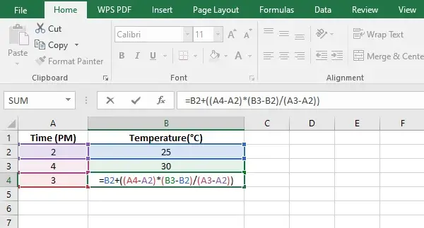
Suppose that you are estimating the temperature of a room at a given time.

At 2:00 PM, the temperature is 25 Celcius.

At 4:00 PM, the temperature is 30 Celcius.

Now, we want to estimate the room temperature at 3:00 PM. 

Method 1: Using the Mathematical Formula for Linear Interpolation in Excel

Step 1: Enter the data into the Excel sheet.

We will enter the data in the Excel sheet.

In cell A1, type Time (PM).

In cell B1, type Temperature (Celcius).

Now enter the time and the temperature in the A column and B column respectively.

Step 2: Entering the interpolation formula

Enter the time for which you want to know the temperature in A4

Enter the formula to calculate the temperature in B4.

B4 =B2 + ((A4 – A2) * (B3 – B2) / (A3 – A2))

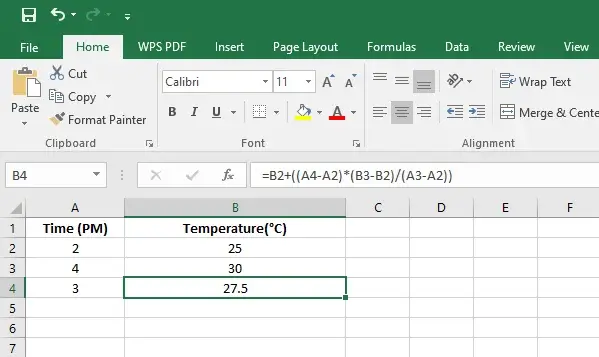
Step 3: Executing the Formula:

Press Enter in cell B4 to see the interpolated result at 3 PM.

Now you can see the result; you can change the time to any value in between the known values for the interpolation to work.

Method 2: Using the TREND Function for Linear Interpolation:

This method is useful for data analysis as it can generate multiple interpolated values in one go. This method assumes a linear relationship hence it is ideal for linearly changing data and not optimal for data with a non-linear relationship.

Let’s take another example:

Example:

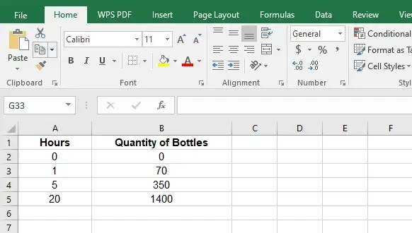
Suppose that you are managing a production line and tracking the number of bottles being manufactured in hours in a day. The table below shows the production quantity

Hours 

Bottles being manufactured against time
Hours	Quantity of Bottles
0	0
1	70
5	350
20	1400

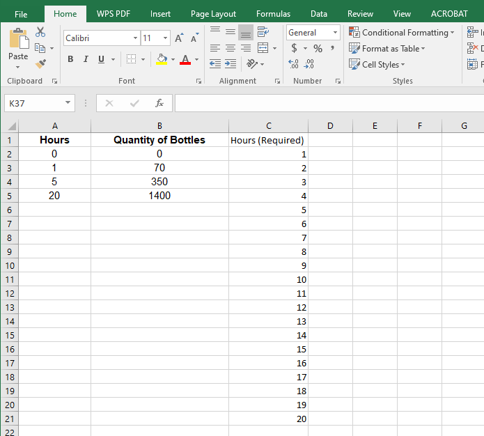
Now, you want to interpolate the output for every hour of production.

Step 1: Input the Data

In cell A1, type Hours

In cell B1, type Quantity of Bottles

Now enter the hours and the quantity of bottles. 

Step 2: Write the interpolation points

In the column C, list the hours you want to interpolate for. In this case, the hours from 0 to 20 are to be interpolated.

Step 3: Apply the TREND Function

Now enter the TREND Formula in cell D2

The formula becomes:

=TREND(B2:B5, A2:A5, C2:C21)

Where values:  B2:B5 are the known quantity of bottles.

A2:A5 are the known hours.

C2:C21 are for which quantity of bottles is required

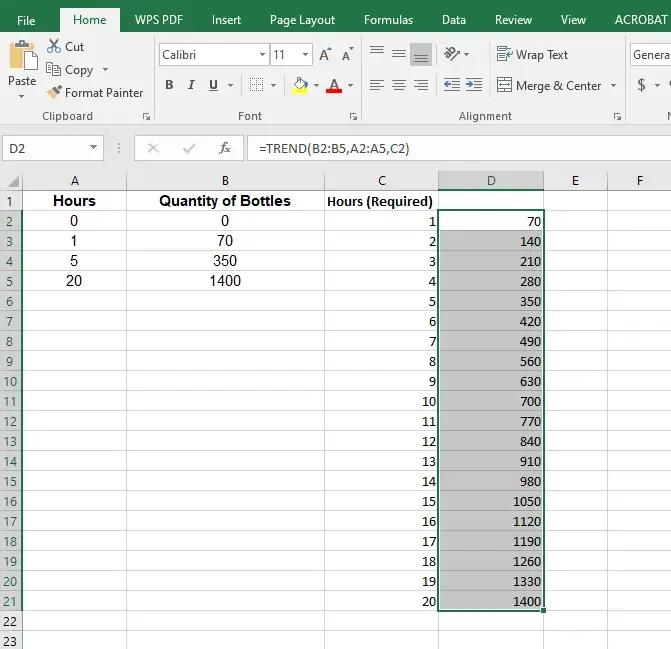
Now put the same formula against all the required hours in column D2:D21

Here you can see the number of bottles manufactured at each hour calculated using linear interpolation in excel.

Method 3: Linear Interpolation in Excel using FORECAST.LINEAR Function.

This function is used for linearly changing data and can predict future values as well. 

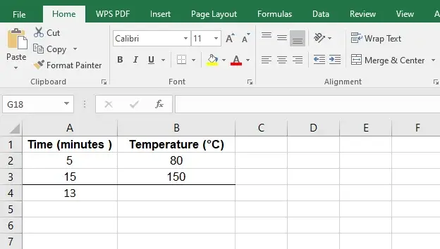
Suppose an example: The temperature of the oven is increasing with time. 

We want to know the temperature of the oven at 13 minutes.

Time (minutes )	Temperature (Celcius)
5	80
15	150
13

Step 1: Input the Data

Input the data in an Excel sheet.

Step 2: Use FORECAST.LINEAR

Click on the cell where you want to see the interpolated result, in this case, it is cell B4.

Write down the formula, in this case

=FORECAST.LINEAR(13, B2:B3,A2,A3)

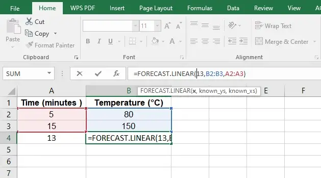
Where 13 is the value at which we want to interpolate, B2:B3 are the values for temperature and A2:A3 are the corresponding temperatures at those times.

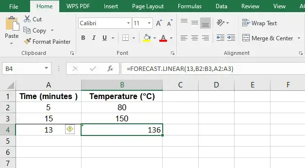
Step 3: Execute the Formula:

Now Enter to calculate the interpolated value in cell B4.

Method 4: Performing Linear Interpolation using a Scatter Plot with Trendline

A scatter plot can also be used for Linear Interpolation in Excel, using an example, we will create a scatter plot in Excel.

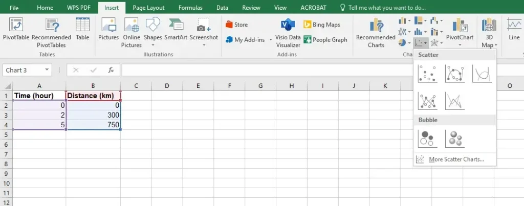
Suppose we are measuring the distance a train travels. We have two data points. 

Time (hour)	Distance (km)
2	300
5	750

Step 1: Input the Data

Input the data as done in previous methods. 

Step 2: Create the Scatter Plot

Select the data by highlighting it, in this case, highlight from cells A1:B3

Then go to Insert > Scatter Plot > Choose Scatter 

Select a line graph.

Step 3: Add a Trendline

Click on the chart to make the chart tools appear, Add a trendline from there.

Go to the chart design tab > Click Add Chart Element > Hover over the Trendline and select Linear.

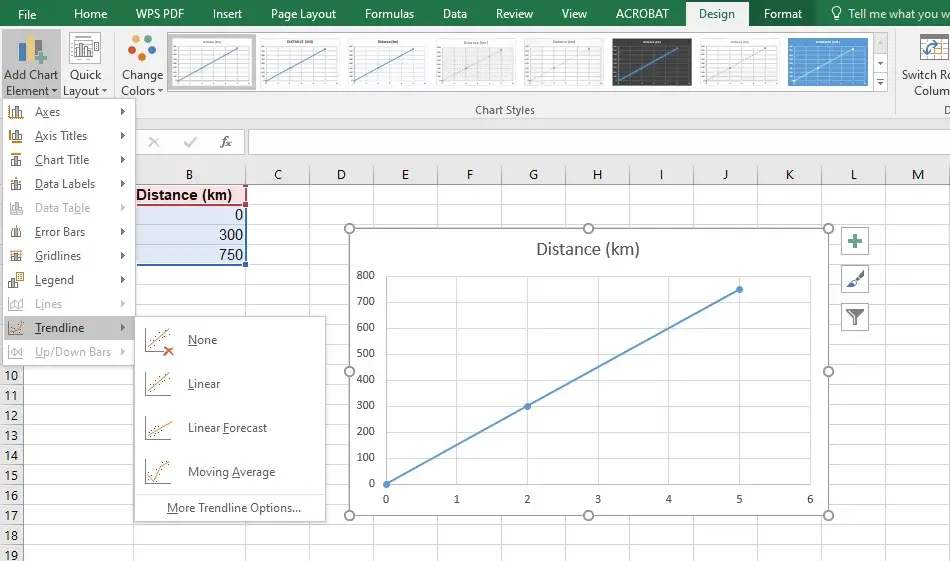
Step 4: Use the equation for interpolation

Go to Quick Layouts and check the option which shows the formula on the line.

Now you can see the equation of the line, which can be used to calculate any point.

In this case.

y=150x. 

Where y is the distance in km

x is the time in hours.

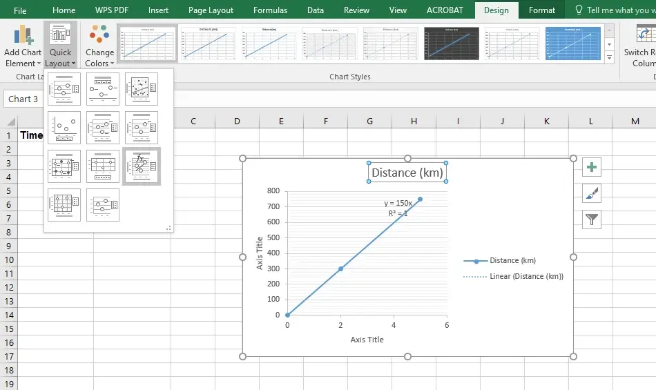
Using this equation, you can put any value at which you want to interpolate, just solve the equation to find the interpolated result.

These are some of the methods by which you can perform Linear Interpolation in Excel. It should be noted that these methods work well for linearly changing data and may result in errors if these methods are used for non-linear data.