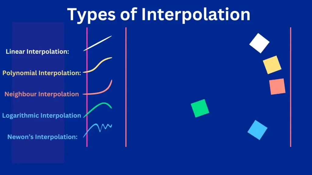
Types of Interpolation: Explained in Detail

Types of Interpolation

Interpolation is a mathematical technique that has been used for a considerable time to calculate unknown values within a discrete data set. Various techniques have been developed for different kinds of data with unique applications. Understanding the types of interpolation and their use cases is crucial for accurately identifying and applying them in calculations. 

Today, we will discuss the various types of interpolation techniques used in the field of mathematics.

Linear Interpolation:

This is the easiest and most widely used interpolation technique. Linear Interpolation is used for data points that are in a straight line and have a linear relationship. 

The formula for Linear Interpolation is as follows:

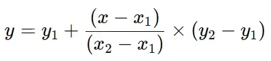
Where (x1, y1) and (x2, y2) are the known data points,

x is the point where the unknown value exists.

y is the unknown value and hence the interpolated result at x.

Applications:

• Used for image scaling.
• Approximation of values in experimental analysis.
• Used to estimate elevation between known points on the Earth.

Advantages	Disadvantages:
The simplest interpolation technique to apply.	The final interpolated values may not provide a smooth line.
Provides a unique solution for a given value.	Not suitable for data with high variability.
Less computational resources are required.	Tend to produce a high error on the edges.

Polynomial Interpolation:

Polynomial interpolation is done by constructing a polynomial function that fits a single polynomial P(x) of degree n through n+1 data points (x0,y0), (x1, y1),…, (xn,yn). 

One common form of the interpolating polynomial is the Lagrange form:

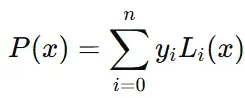
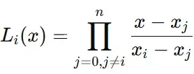
 Where Li(x) are the Lagrange basis polynomials, defined as:

Another method is Newton’s divided differences. Newton’s method constructs the polynomial iteratively.

Where f(x0,x1,…) are the divided differences.

Applications:

• It can be used for smoothing and curve fitting
• Used for designing smooth animations in transitions.
• Approximating functions between known data points.

Advantages:	Disadvantages:
Produces a smooth and continuous function.	Computationally more demanding to solve.
It can provide an explicit formula for the interpolating function.	One data point can affect the entire polynomial.
Pass through all provided data points.	Even small changes in data can lead to large changes in the interpolated polynomial.

Spline Interpolation:

It uses splines to interpolate the data. The most common spline is the cubic spline, which is a third-degree polynomial used between each pair of data points. 

For intervals (xi, xi+1), the cubic slime is defined as: 

Applications:

• This technique is used in data visualisation to create smooth plots through data points.
• It’s used in path planning for robots.
• Used to reconstruct smooth curves in anatomical structures during medical imaging.

Advantages:	Disadvantages:
This technique creates a smooth and continuous curve.	Requires more resources to compute.
Unwanted oscillations are not introduced using this interpolation.	Requires solving a system of equations.
A large amount of data is easily processed.	It can be less accurate when used for data containing sharp corners and/or discontinuous data.

Nearest-Neighbour Interpolation:

This technique is used by assigning the value of the unknown point to the nearest known data point.

Applications:

• For image processing when resizing is required.
• Used in medical imaging for reconstructing images from a scan.
• Used for handling missing data while analysing data.

Advantages:	Disadvantages:
Less computational resources are required.	Tends to produce blocky artifacts when used in images.
Original values and data are preserved.	It is not ideal for applications where smooth data transition is required.
Data distribution assumption is not required.	Neighbouring data points are ignored, which can lead to errors.

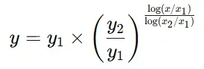
5) Logarithmic Interpolation:

This interpolation technique is used for data exhibiting logarithmic trends. For two given points. (x1, y1) and (x2, y2)

Applications:

• Used in estimating population growth.
• Used for estimating the magnitude of the earthquakes.
• Used in Audio Engineering.

Advantages:	Disadvantages:
Best interpolation technique for data following a logarithmic or an exponential trend.	Not applicable for non-logarithmic data.
The technique is praised for handling a large range of data effectively.	Computationally more resource-consuming.
In data where the relationship is multiplicative, distortion is reduced.	It can create errors in data which is incorrectly sampled.

6) Newton’s Interpolation:

Newton’s divided difference formula is as follows:

Applications:

• Used in data analysis for polynomial fitting.
• Used for weather modelling.
• Useful for interpolating data points in engineering problems. 

Advantages:

Disadvantages:

7) Lagrange Interpolation:

Lagrange interpolation is a numerical method in which a function is approximated that passes through a given set of points. In Lagrange interpolation, the polynomial that passes through the points is of degree n-1 where n is the number of data points. So for example, if there are 5 data points, the polynomial made by Lagrange interpolation will be a 4th degree polynomial. 

For a given set of n data points (x0,y0), (x1, y1),…, (xn,yn),  the Lagrange polynomial is given by:

Where Li (x) is the Lagrange basis polynomial, defined as 

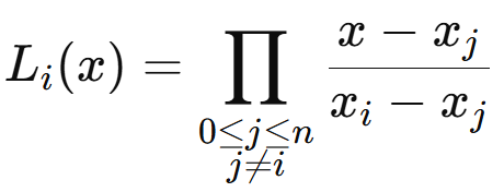
• Here, P(x) is the interpolated polynomial.
• yi are the known values of the function at xi
• Li (x) is the Lagrange basis polynomial for each data point.

Applications:

• Data Estimation.
• Predictive modelling for weather forecasting.
• Rendering and texture mapping in computer graphics.

Advantages:

• Highly accurate for small data sets.
• Ability to fit a single polynomial to multiple data values.
• It can provide exact results at a given point.

Disadvantages:

• When a large dataset with equally spaced points is used, large oscillations at endpoints, called Runge’s phenomenon, can occur. 
• It requires significant computational resources to solve.

Conclusion

Interpolation is a useful mathematical technique used to estimate values between known data points, from simple methods like linear interpolation to more complex techniques namely spline interpolation and Lagrange interpolation. Each methods have their own advantages and disadvantages.

Polynomial interpolation allows for smooth approximation, while nearest-neighbour is a simple method for fast estimation, Logarithmic and Lagrange’s interpolation are suited for specific data types requiring more complexity to estimate. 

Choosing the appropriate interpolation technique can determine whether your estimations are accurate or flawed. By familiarizing yourself with these techniques, you can select the method that best meets your needs.